Machine learning Gradient Descent Code for Linear Regression Course1 Week 1 Final

原jupytar notebook地址： https://www.coursera.org/learn/machine-learning/ungradedLab/lE1al/optional-lab-gradient-descent/lab?path=%2Fnotebooks%2FC1_W1_Lab04_Gradient_Descent_Soln.ipynb

分析：

一。 导入库 import

二。定义训练数据 load data set ——features&target value

三。定义代价函数 def compute_cost（x,y,w,b)

四。计算梯度 （求偏导数）

这部分需要复习求偏导知识

b与x没有乘积关系 求偏导时与x无关

有了偏导函数 可以遍历dj-dw和dj-db 注意要同时赋值

右边这个梯度方向场 箭头向右 梯度为正，箭头向左 剃度为负 为零是为一个点

五。 绘制梯度图

六。计算梯度下降

记录所有

迭代更新w、b 记录历史数据 alpha是学习率

减少打印次数：如果每次迭代都 print，会产生大量输出，影响运行效率。

监控训练进度：每 10% 迭代一次，可以观察 Cost（损失）是否下降，w 和 b 是否趋于稳定。

避免过拟合：如果 Cost 下降变慢或趋于平稳，可以考虑调整学习率或者减少训练次数。

.2e：科学计数法格式，保留 2 位小数。例如：

• 12345.6789 变成 1.23e+04

• 0.00056789 变成 5.68e-04

七。运行梯度下降

给初始值w=0， b=0，iterations=10000 迭代次数

tmp-alpha=1.0e-2 即0.01

会得到一组w b的值

八：检测梯度下降是否收敛

左图是早期损失的变化 右图是晚期的变化

1. 查看梯度下降是否收敛

   • 如果右图（后期）损失值趋于平稳 → 说明优化已收敛 

   • 如果右图仍然震荡或下降很慢 → 可能需要调整学习率 

2. 观察训练初期损失下降趋势

   • 如果初期下降很快 → 说明梯度下降有效

   • 如果初期损失没有下降或波动剧烈 → 可能需要调整超参数（如学习率）

九。预测数值

输入想要预测的x的值 会得到对应的y

十。观察损失下降的步长变化

红色箭头代表的步长越来越小

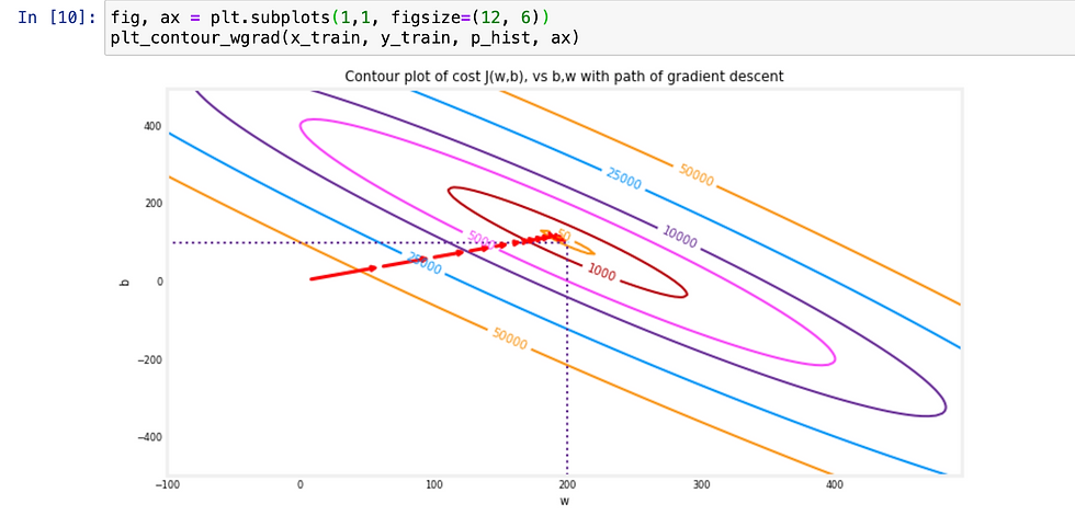
Above, the contour plot shows the 𝑐𝑜𝑠𝑡(𝑤,𝑏)cost(w,b) over a range of 𝑤w and 𝑏b. Cost levels are represented by the rings. Overlayed, using red arrows, is the path of gradient descent. Here are some things to note:

• The path makes steady (monotonic) progress toward its goal.

• initial steps are much larger than the steps near the goal.

Zooming in, we can see that final steps of gradient descent. Note the distance between steps shrinks as the gradient approaches zero.

邻近圆心时的步长变化 图例放大了